 |

This is a follow-up on the first LPCNet demo. In the first demo, we presented the LPCNet architecture, combining signal processing and deep learning to improve the efficiency of neural speech synthesis. This time, we turn LPCNet into a very low-bitrate neural speech codec (see submitted paper) that's actually usable on current hardware and even on phones. It’s the first time a neural vocoder is able to run in real-time using just one CPU core on a phone (as opposed to a high-end GPU). The resulting bitrate — just 1.6 kb/s — is about 10 times less than what wideband codecs typically use. The quality is much better than existing very low bitrate vocoders and comparable to that of more traditional codecs using a higher bitrate.
There are two broad types of speech codecs: waveform coders and vocoders. Waveform coders include Opus, AMR/AMR-WB, and all the codecs that can be used for music. They attempt to make the decoded waveform as close as possible to the input — usually with some perceptual considerations. Vocoders on the other hand are really synthesizers. The encoder extracts information about the pitch and the shape of the vocal tract, transmits that information to the decoder, and then the decoder resynthesizes a new speech signal based on what the encoder provided. It's almost like doing speech recognition in the encoder and then text-to-speech in the decoder, except that the encoder's a lot simpler/faster than a speech recognizer (and it transmits a bit more information).
Vocoders have been around since the 70s, but because their decoders are doing something similar to speech synthesis, they couldn't really be much better than the speech synthesis systems, which sounded pretty awful until recently. That's why vocoders were generally used at bitrates below around 3 kb/s. Above that, waveform coders just sound better. Things stayed like that until recently when neural speech synthesis systems like WaveNet appeared. Suddenly synthesis started sounding a lot better and, sure enough, someone soon decided to turn WaveNet into a vocoder.
WaveNet can produce very high quality speech, but that comes at a cost in complexity — in the hundreds of GFLOPS. LPCNet manages to significantly reduce that complexity. It builds on WaveRNN, which already improves on WaveNet by using a recurrent neural network (RNN) and sparse matrices. LPCNet further improves on WaveRNN by using linear prediction (aka LPC). LPC is the part of old vocoders that did work well. It predicts a sample from a linear combination of the previous samples and — most importantly — does so at a cost that's negligible compared to that of a neural network. Of course it can't do everything (otherwise 70s vocoders would have sounded great), but it can take a lot of the load away from the neural network. That makes it possible to use a smaller network than WaveRNN and still achieve the same quality.
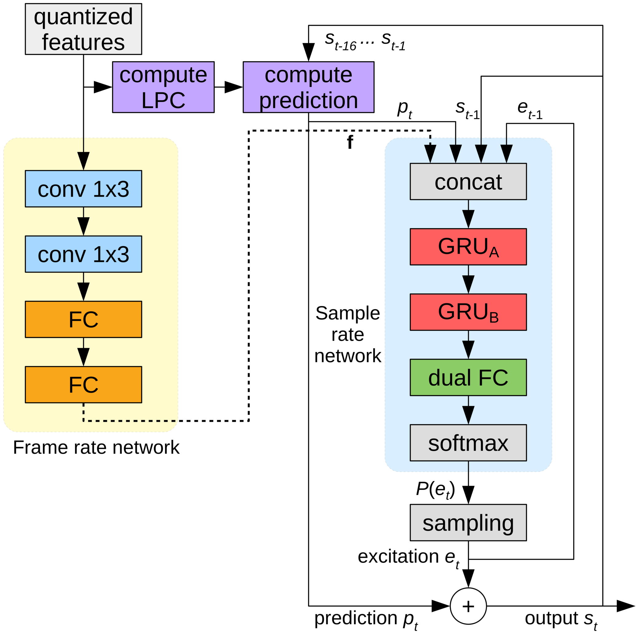
LPCNet synthesizes speech from vectors of 20 features every 10-ms frame. Of the 20 features, 18 are cepstral coefficients representing the shape of the spectrum. The two others describe the pitch of the voice: one parameter for the pitch period, and one for its strength (how correlated the signal is with itself when delayed by the pitch period). When stored as floating-point values, these features take up 64 kb/s to store or transmit. That's not very useful considering that a codec like Opus produces very high quality speech at just 16 kb/s (for 16 kHz mono). Clearly we need to apply some heavy compression here.
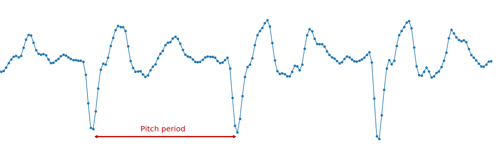
All pitch codecs rely heavily on pitch, but unlike waveform coders where pitch "just" helps reducing the amount redundancy, vocoders have no fallback and will generate bad-sounding (or even unintelligible) speech if the pitch is wrong. Without going into the details (see the paper), the LPCNet encoder is trying hard to not to get the pitch wrong. The search starts by looking for correlations in the speech signal across time. See below how a typical pitch search works. ▶ Show nerdy details ▼ Hide nerdy details OK, we're omitting one detail here. In practice, we don't search for the pitch directly on the signal, but rather on the prediction residual aka excitation, which similar to what the speech would be without the vocal tract. Because the residual is white (i.e. it has about the same amount of energy at all frequencies), the correlation used in the pitch search has a much narrower peak, making it easier to pick the exact period.
Once we know what the pitch is, we need to code the information with as few bits as possible, without making the output sound significantly worse. Because we naturally perceive frequency on a log scale (e.g. each octave in music represents a factor of two in frequency), encoding the log of the pitch makes sense. The speaking pitch of most people (we're not trying to capture a soprano singing here) falls between 62.5 Hz and 500 Hz. With 7 bits (128 possible values), we can have a resolution around one quarter-tone (the difference between and C and a D is one tone).
So we're done with pitch, right? Well, not so fast. Humans don't speak like 1960s movie robots. Instead, our pitch can vary over time — even during a 40-ms packet. So we need to take that into account by coding a pitch variation parameter: 3 bits to code a difference of up to 2.5 semitones between the beginning and the end of the packet. The last thing we need to code is the pitch correlation itself. The correlation is how strong the pitch is, differentiating between vowels and unvoiced consonants (e.g. s and f). Just two bits are enough for the correlation.
While pitch contains information about how something is said (prosody, emotion, emphasis, ...), it's the spectral envelope that determines what was said (except for tonal languages like Chinese for which pitch is really important). What's produced by the vocal cords is about the same for any vowel. It's how we shape our vocal tract that determines which sound we're making. The vocal tract acts like a filter and the encoder's job is to estimate that filter and transmit it to the decoder. This can be done efficiently by converting the shape of the spectrum into a cepstrum (yes, that's "spectrum" reversed, that's how funny us DSP people think we are).
For 16 kHz input, the cepstrum we use is basically a vector of 18 numbers every 10-ms that we need to shrink as much as possible. Because we have 4 of those vectors in a 40-ms packet and they tend to be similar to each other, we want to do our best to reduce the redundancy as much as possible. This can be done by using the neighboring vectors as predictors and only transmitting the difference between the prediction and the real value. At the same time, we also don't want to depend too much on previous packets in case one of them goes missing. Sounds like a problem someone's already solved...
If all you have is a hammer, everything looks like a nail — Abraham Maslow.
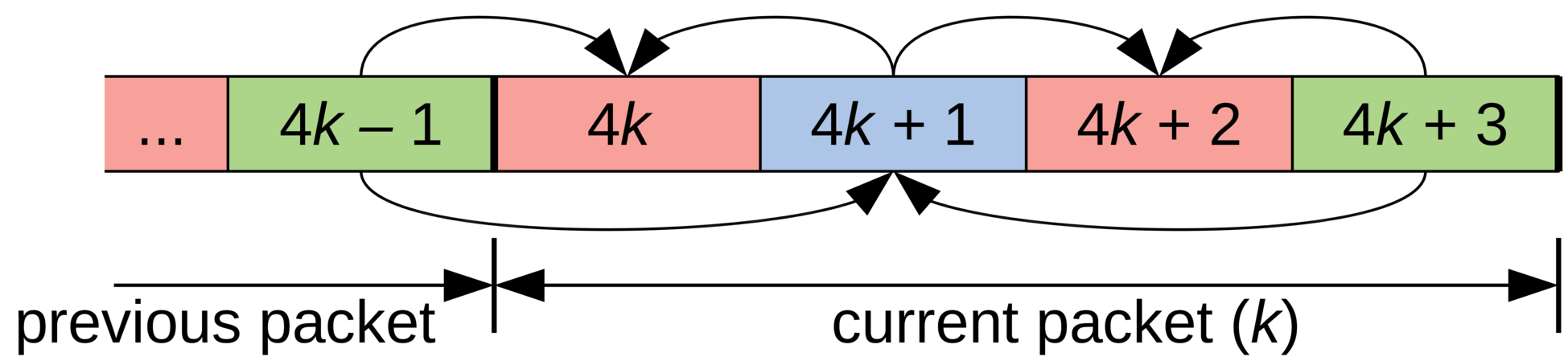
And if you spent a few years working on video codecs, then you're bound to see B-frames somewhere. Unlike video codecs that often split frames in many packets, here we need to encode many frames in one packet. So we start by coding a keyframe, i.e. an independent vector, and the end of the packet. That vector is coded without prediction, using 37 bits: 7 for the overall energy (the first cepstral coefficient) and 30 bits for the rest, using vector quantization (VQ). Then comes the (hierarchical) B-frames. We can use two keyframes (the one from the current packet and the one from previous packet) to predict the cepstrum that's at the mid-point between them. We can decide to pick any of the two keyframes, or their average, as the predictor before encoding the difference between the real value and the prediction. We use VQ again and code that vector using a total of 13 bits, including selecting the predictor. At that point, we're left with just two vectors and very few bits. We use our last 3 bits to just select a predictor for these remaining vectors. Of course, it's much easier to visualize than read, so see the figure below.
Adding up all the bits listed above, we get 64 bits per 40-ms packet, or 1600 bits per second. For those who like to think in terms of compression ratio, uncompressed wideband speech is 256 kb/s (16 kHz x 16 bits/sample), which means a compression ratio of 160x! Of course, it's always possible to play with the quantizers to get either lower or higher bitrates (with the corresponding effect on quality) but hey, we have to start somewhere. See below a summary of where all the bits are going.
| Bit Allocation | |
| Parameter | Bits |
| Pitch period | 6 |
| Pitch modulation | 3 |
| Pitch correlation | 2 |
| Energy | 7 |
| Independent cepstrum VQ (40 ms) | 30 |
| Predicted cepstrum VQ (20 ms) | 13 |
| Cepstrum interpolation (10 ms) | 3 |
| Total | 64 |
The LPCNet source code is available under a BSD license. It includes a library that makes it easy to use the 1.6 kb/s codec. Note that neither the format, nor the API is frozen. Both will change in the future. The repository also includes an lpcnet_demo example application that makes it easy to just test the codec from the command line. See the README.md file for complete instructions.
For those who want to go a bit deeper, it's also possible to train new models and/or use LPCNet as a building block for other applications, such as text-to-speech (LPCNet is just one component of TTS, it doesn't do TTS all by itself).
Neural speech synthesis can be quite CPU-intensive. At last year's ICASSP, Bastiaan Kleijn and his colleagues at Google/DeepMind presented a 2.4 kb/s WaveNet-based codec that used the codec2 bitstream. While it sounded amazing, its complexity — in the hundreds of GFLOPS — meant there was no way to run it in real-time without a high-end GPU and a lot of effort.
By contrast, the complexity of this 1.6 kb/s LPCNet-based codec is just 3 GFLOPS and it's designed to run in real-time on much more accessible hardware and actually be shippable in applications today. To get good performance, we had to write some AVX2/FMA and Neon code (intrinsics only, no assembly). With that, we're now able to code (and especially decode) speech in real-time not only on PC, but also on most recent phones. See below the performance we got on both x86 and ARM CPUs.
| Performance | |||
| CPU | Clock | % of one core | Real-time |
| AMD 2990WX (Threadripper) | 3.0 GHz* | 14% | 7.0x |
| Intel Xeon E5-2640 v4 (Broadwell) | 2.4 GHz* | 20% | 5.0x |
| Snapdragon 855 (Cortex-A76 on Galaxy S10) | 2.82 GHz | 31% | 3.2x |
| Snapdragon 845 (Cortex-A75 on Pixel 3) | 2.5 GHz | 68% | 1.47x |
| AMD A1100 (Cortex-A57) | 1.7 GHz | 102% | 0.98x |
| BCM2837 (Cortex-A53 on Raspberry Pi 3) | 1.2 GHz | 310% | 0.32x |
| *turbo enabled | |||
The numbers are quite interesting. On x86, while we're only showing Broadwell and Threadripper, Haswell and Skylake have similar performance (when accounting for the clock). On the ARM side though, clearly not all cores are created equal. Even when accounting for the clock difference, the A76 is still 5-6 times faster than the A53, which is expected since the A53 is mostly used as a power-efficient core (e.g. in big.LITTLE systems). Still it means that LPCNet can now run in real time on a modern phone while using just one core. Having LPCNet run in real-time on the Raspberry Pi 3 would be nice too. For now it's nowhere near real-time, but that doesn't mean it's impossible either.
On x86, the exact cause of the performance limitation at ~1/5 of the theoretical peak performance is still a mystery. Matrix-vector products are known to be less efficient than matrix-matrix products because they require more loads per operation — more specifically, one load from the matrix for each FMA operation. On the one hand, performance appears to be related to the L2 cache providing only 16 B/cycle. On the other hand, Intel claims that the L2 can provide up to 32 B/cycle on Broadwell and 64 B/cycle on Skylake. ▶ Show nerdy details ▼ Hide nerdy details Those who inspect the current code closely may notice another bottleneck: the fact that the FMA operations reuse the same sum and only allow 2 FMAs in flight at any time. That bottleneck is easy to fix with partial sums, but fixing it does not improve performance (because of some other bottleneck as discussed above), so we keep the code like it is until the other bottlenecks are fixed.
We ran a MUSHRA-like listening test to see how LPCNet compares to other codecs. These are the conditions tested:
In a first test (Set 1), we had 8 utterances from 2 male and 2 female speakers. The files in Set 1 belong to the same database (i.e. same recording conditions) that was used for training, but the speakers used for testing were excluded from the training set. In a second test (Set 2), we used some of the files used for the Opus test vector (not compressed), recording in different conditions just to make sure that LPCNet can generalize a bit. Both tests had 100 participants, which is why the error bars are rather small. See the results below.

Overall, 1.6 kb/s LPCNet looks good — much better than MELP at 2.4 kb/s, and not so far behind Opus running at 9 kb/s. The fact that the unquantized LPCNet model has slightly better quality than 9 kb/s Opus, means there's room for higher quality if we're willing to consider bitrates in the 2-6 kb/s range.
Here are three of the samples that were used in the listening test above.
Select sample
Select algorithm
Select where to start playing when selecting a new sample
Player will continue when changing sample.
Comparing the quality of compressed and uncompressed LPCNet with Opus, MELP, and Speex. This demo requires a browser that supports FLAC or WAV playback in HTML5.
We think this is cool technology in itself, but it also has real-world applications. Here are just some of the possibilities.
Not everyone is fortunate enough to always have access to a high-speed connection. In some places in the world, service is sometimes very slow and highly unreliable. Being able to code reasonable quality speech at 1.6 kb/s means being able to work in those conditions and even being able to transmit packets multiple times (for increased robustness) while still within the small bandwidth budget. Of course, because of the overhead of packet headers (40 bytes for IP+UDP+RTP), we actually want packets of at least 40, if not 80 or 120 ms.
For the past 10 years, David Rowe has been working on transmitting digital voice over the air. He created Codec2, which can be used to code speech at bitrates ranging from just 700 b/s to 3.2 kb/s. For the past year, David and I have been discussing how to improve Codec2 using neural synthesis, and with LPCNet we're now finally getting there. Read David's latest blog post for samples of his own LPCNet-based codec implementation, which is meant to be integrated with FreeDV.
Being able to encode a decent-quality bitstream in very few bits can be useful for transmitting redundancy when dealing with an unreliable network connection. Opus already includes a forward error correction (FEC) mechanism known as LBRR, which codes a low-bitrate version of the previous frame and sends it in the current frame. It works well, but adds a significant overhead. Having a redundant stream transmitted at just 1.6 kb/s would be a lot more efficient and would even allow including more redundancy.
There are still many possibilities and applications that have not been explored. One interesting area would be to use LPCNet to enhance an existing codec (like Opus). Like other codecs, the quality of Opus degrades rather quickly when going to very low bitrates (e.g. < 8 kb/s) because there aren't enough bits to match the input signal (remember, waveform coders attempt to do that). However, the linear prediction information already transmitted by the encoder may be enough for LPCNet to synthesize decent-sounding speech — possibly better than what Opus can do at these bitrate. On top of that, the rest of the information Opus transmits (prediction residual) may be able to help LPCNet synthesize an even better output. In some sense, LPCNet could be adapted to work as a fancy post-filter to improve the quality of Opus (or any other code) without the need to change the bit-stream (i.e. preserving complete compatibility).
If you would like to comment on this demo, you can do so on on my blog.
—Jean-Marc Valin (jmvalin@jmvalin.ca) March 29, 2019