

Perceptual vector quantization (PVQ), along with the lapped transforms, is one of the key techniques in Daala that forces us to do everything else differently from other video codecs. It is also one of the least intuitive and hardest to visualize techniques we have right now. Hopefully, this demo will help demystifying how it works using only the minimal amount of math.
If all you have is a hammer, everything looks like a nail — Abraham Maslow.
One of the key characteristics of CELT (one of the two coding techniques in Opus) is the constrained energy (first two letters of CELT) approach. The idea is to directly encode the amount of audio energy as a function of frequency and then separately encode how that energy is distributed in time and frequency. This leads to interesting perceptual properties (more about CELT in this paper). If you are an audio codec developer, everything looks like an audio signal.
So PVQ is an attempt at transposing the constrained energy idea to video. Instead of audio energy, we attempt to preserve contrast.
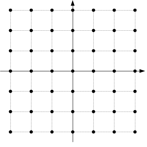
The vast majority of video and still image codecs use scalar quantization.
That is, once the image is transformed into frequency-domain coefficients,
each (scalar) coefficient is separately quantized to an integer index. Each
index represents a certain scalar value that the decoder will use to
reconstruct the image. For example, using a quantization step size of
(e.g.) 10, a decoder receiving indices -2, +4, will reconstruct
-20, +40, respectively. Scalar quantization has the advantage that each
dimension can be quantized independently from the others.
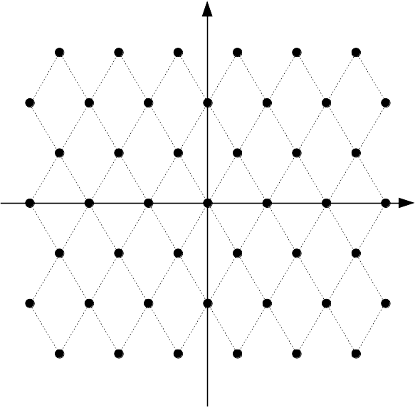
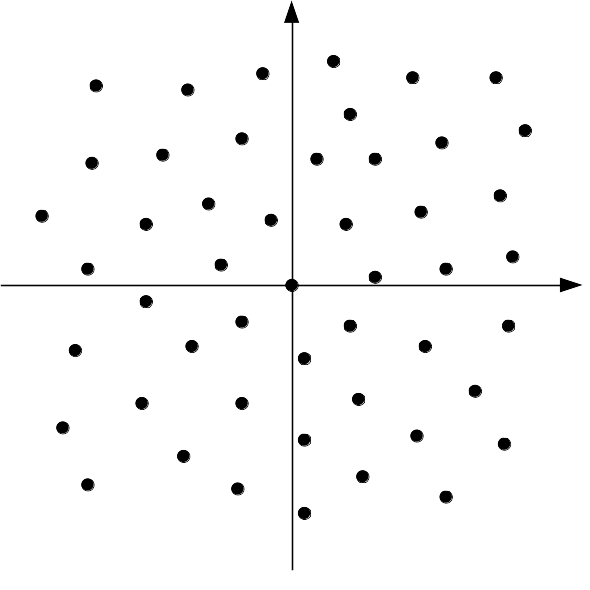
With vector quantization, an index no longer represents a scalar value, but an entire vector. The possible reconstructed vectors are no longer constrained to the regular rectangular grid above, but can be arranged in any way we like, either regularly, or irregularly. Each possible vector is called a codeword and the set of all possible codewords is called a codebook. The codebook may be finite if we have an exhaustive list of all possibilities or it can also be infinite in cases where it is defined algebraically (e.g., scalar quantization is equivalent to vector quantization with a particular infinite codebook)
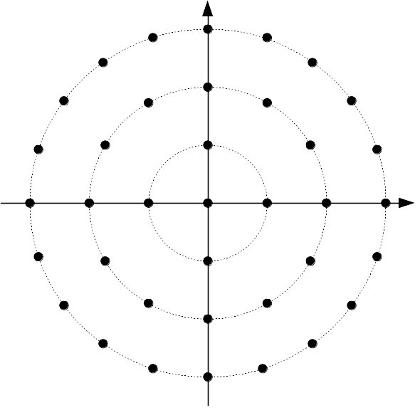
The idea of gain-shape vector quantization is to represent a vector by separating it into a length and a direction. The gain (the length) says how much energy is in the vector. The shape (the direction) says where in the vector that energy is concentrated. In two dimensions, one can construct a gain-shape quantizer using polar coordinates, with gain being the radius and the shape being the angle. In three dimensions, one option (there are many more) is to use latitude/longitude for the shape. In Daala, we don't restrict ourselves to just two or three dimensions. For a 4x4 transform, we have 16 DCT coefficients. We always code the DC separately, so we are left with a vector of 15 AC coefficients to quantize. If we did this with scalar quantization, we would have to code 16 values to represent these 15 coefficients: the 15 individual coefficients plus the gain. That would be redundant and inefficient. But by using vector quantization, we can code the direction of an N-dimensional vector with (N - 1) degrees of freedom, just like we did with polar coordinates in 2-D and latitude and longitude in 3-D. It's OK if you cannot visualize 15-dimensional spaces — nobody can. Normally, we just visualize the first two or three and generalize from there.
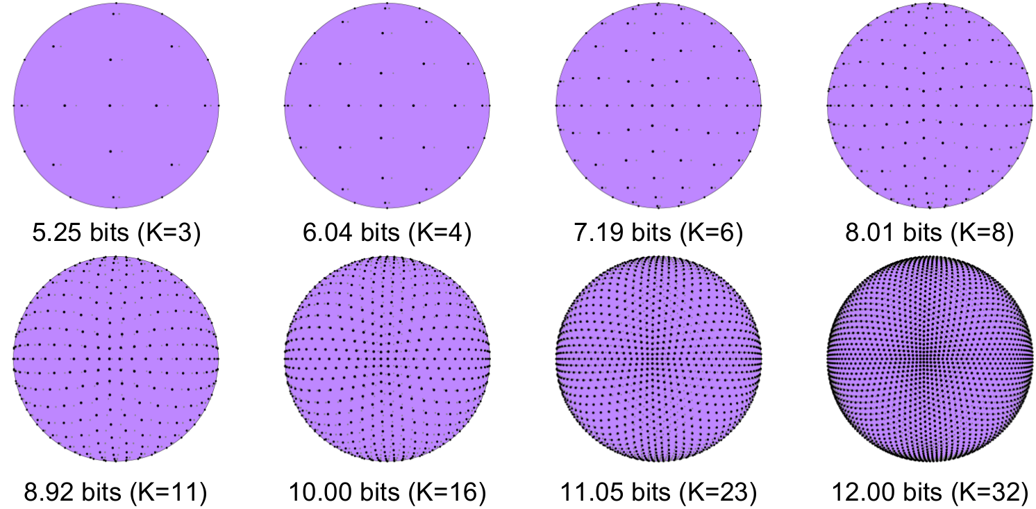
In Daala, just like in CELT, the shape codebook we use is a normalized version of the pyramid vector quantizer described by Fischer in 1986. Fischer's codebook is defined as the set of all N-dimensional vectors of integers where the absolute value of the integers sum to K. K is called the number of pulses because you can think of building such a vector by distributing K different pulses of unit amplitude, one at a time, among the N dimensions. The pulses can point in either the positive or negative direction, but all of the ones in the same dimension must point in the same direction. For N=2 and K=2, our codebook has 8 entries:
(2, 0), (-2, 0), (1, 1), (1, -1), (-1, 1), (-1, -1), (0, 2), (0, -2)
The normalized version of the codebook simply normalizes each vector to have a length of 1. If y is part of Fischer's non-normalized codebook, then the corresponding normalized vector is simply y/||y||2.
The advantage of this codebook is that it is both flexible (any value of K will work), and easy to search. Its regularity means that we don't have to examine every vector in the codebook to find the best representation for our input.
The number of dimensions, N, is fixed, so the parameter K
determines the quantization resolution of the codebook (i.e., the spacing
between codewords). As the gain of our vector increases, we need more
points on our N-dimensional sphere to keep the same quantization
resolution, so K must increase as a function of the gain. In the
example below, K is set to provide about the same quantization
resolution irrespective of the gain.
In three dimensions, this is what the codewords look like for various
K values and a constant gain.
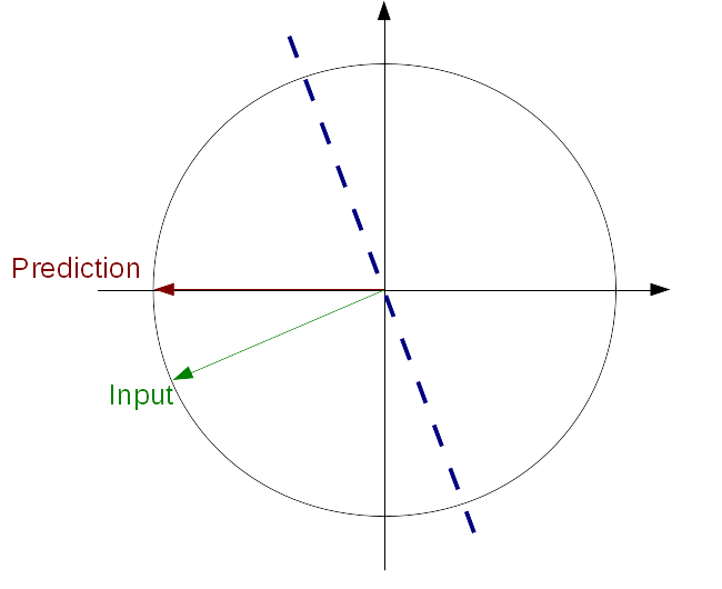
In video coding, we rarely code images from scratch. Instead, we use information from other frames to predict the current frame and in most cases, that prediction turns out to be very good so we want to make sure we make full use of it. Turns out that using prediction with gain-shape quantization is tricky. Tricky enough that I failed twice at integrating pitch prediction in CELT. The naive approach is to just subtract the prediction from the coefficients being coded, and then apply gain-shape quantization to the residual. While this kinda works, we lose the whole point of gain-shape quantization. The gain no longer represents the contrast of the image being coded, but just how much the image changed compared to the prediction. This was the second failed attempt in CELT. The first failed attempt at gain-shape quantization with pitch prediction was a "clever" manipulation of the shape codebook to increase resolution in the region close to the prediction. That turned out to make things quite complicated for very little benefit.
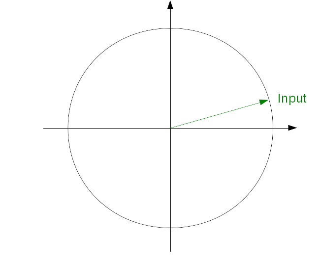
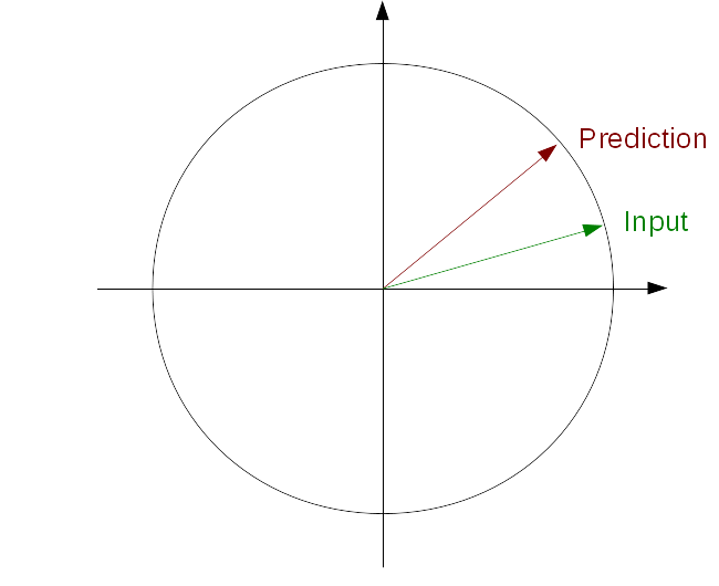
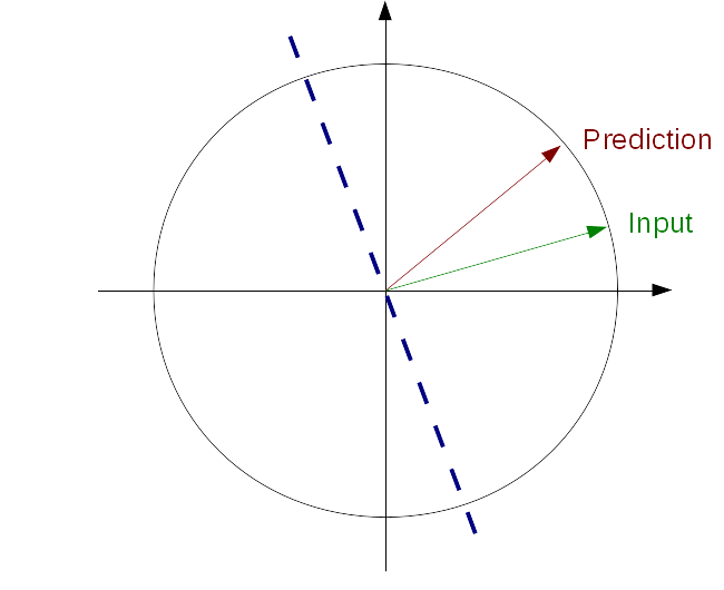
If only we were lucky enough for our prediction to be perfectly aligned with one of our axes, i.e. all but one of its coefficients were zero. Then we could just code the other coefficients from the input and signal what their magnitude is compared to that of the prediction (which is hopefully very small). Turns out we can make our own luck. What we need is some kind of transform that would turn the problem we have into the one we wish we had. This can be done with a Householder reflection. All we need to do is find the reflection plane that turns our prediction into a vector that has only zeros except for a single component.
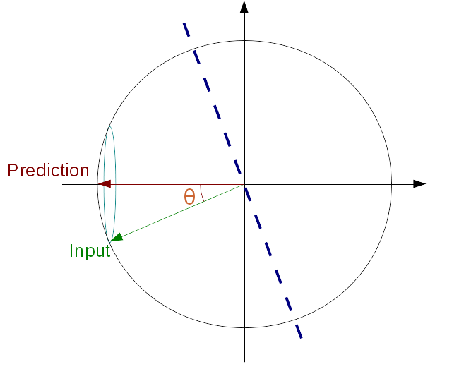
Once our prediction is aligned along an axis, we can code how well it matches our input vector using an angle θ. The position of our input vector along the prediction axis on our hypersphere is simply cos(θ) and the distance between the input and the prediction axis is sin(θ). We can then apply gain-shape quantization to the remaining dimensions, knowing that the gain of the remaining coefficients is just the original gain, multiplied by sin(θ).
This is a step-by-step demonstration of applying prediction to gain-shape quantization

PVQ using prediction. Click on the arrows to see all steps of PVQ with prediction.
Video and still image codecs have long taken advantage of the fact that contrast sensitivity of the human visual system depends on the spatial frequency of a pattern. The contrast sensitivity function is to vision what the absolute threshold of hearing is to audition.
Another factor that influences our perception of contrast is the presence of more contrast at the same location. We call this activity masking. It is the visual equivalent of auditory masking, where the presence of a sound can mask another sound. While auditory masking has been at the center of all audio coding technology since the 80s, the use of activity masking in video coding is comparatively new and less advanced. This is likely due to the fact that activity masking effects are much less understood than auditory masking, which has been the subject of experiments since the 50s (and probably even before that).
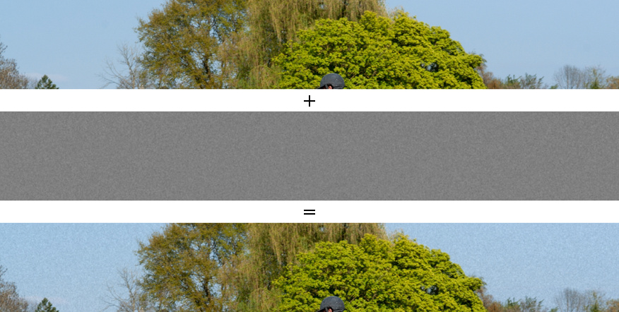
The following is a simple demonstration of activity masking and how
contrast in the original image affects our perception of noise.
Taking into account activity masking has two related, but separate goals:
Together, these two tend to make bit allocation more uniform throughout the frame, though not completely uniform — unlike CELT which has uniform allocation due to the logarithmic sensitivity of the ear.
The idea is that we want to make the quantization noise vary as a function
of the original contrast, typically using a power law. In Daala, we are
trying to make quantization noise follow the amount of contrast raised to
the power α=1/3. We can control the resolution of the shape quantization
simply by controlling the value of K as a function of the gain. Now,
how do we control the resolution of the gain as a function of the gain
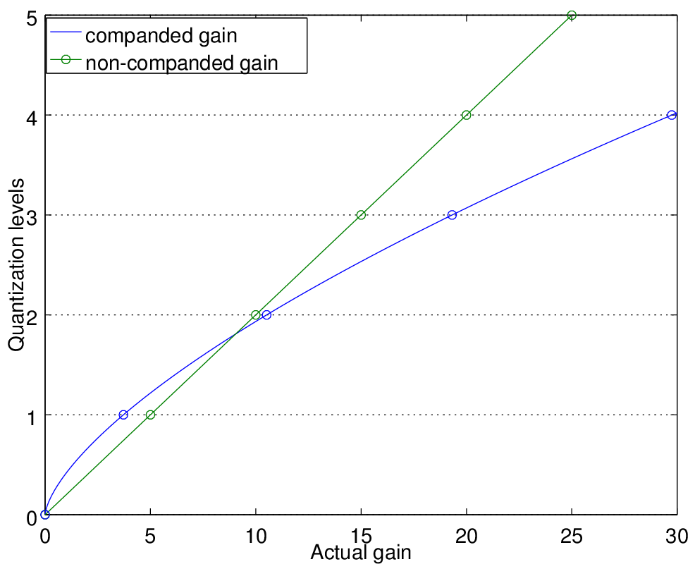
itself? Simply by not encoding the gain itself, but rather a companded version
of it. If we raise the gain to the power (1 - α) and encode the result, we
get better resolution close to gain=0 and worse resolution as the gain
increases, as shown below.
Looking at the actual codebook in 2D, we have:

When using prediction, it is important to apply the gain companding to the original N-dimensional coefficients vector rather than to the N-1 remaining coefficients after prediction. In practice, we only want to consider activity masking in blocks that have texture rather than edges. The easiest way to do this is to consider all 4x4 blocks as having edges and all 8x8 to 32x32 blocks as having texture. Also, we currently only use activity masking for luma because chroma masking is much less understood. For blocks where we disable activity masking, we still use the same quantization described above, but set α=0.
The last thing we need to discuss here is signaling, i.e. how the parameters are transmitted from the encoder to the decoder. The whole point of PVQ is to make activity masking built into the codec, so that no extra information needs to be transmitted. We avoid having to explicitly signal bit-rate changes depending on the amount of contrast like other codecs currently have to do. Better, instead of only being able to signal activity masking rate changes at the macroblock level, we can do it at the block level and even below that. We can treat horizontal coefficients independently of the vertical and diagonal ones, and do that for each octave.
Let's start with the simplest case, where we do not have a predictor. The first parameter we code is the gain, which is raised to the power (1 - α) when activity masking is enabled. From the gain alone, the bit-stream defines how to obtain K, so the decoder knows what K is without the need to signal it. Once we know K, we can code the N-dimensional pyramid VQ codeword. Although it may look like we code more information than scalar quantization because we code the gain, it is not the case because knowing K makes it cheaper to code the remaining vector since we know the sum of the absolute values.
The case with prediction is only slightly more complicated. We still have to encode a gain, but this time we have a prediction, so we can use it to make coding the gain cheaper. After the gain, we code the angle θ with a resolution that depends on the gain. Last, we code a VQ codeword in N - 1 dimensions. Only angles smaller than π/2 allowed, so we code a no reference flag. When set, it means that we ignore the reference and only code the gain and the N-dimensional pyramid VQ codeword (no angle).
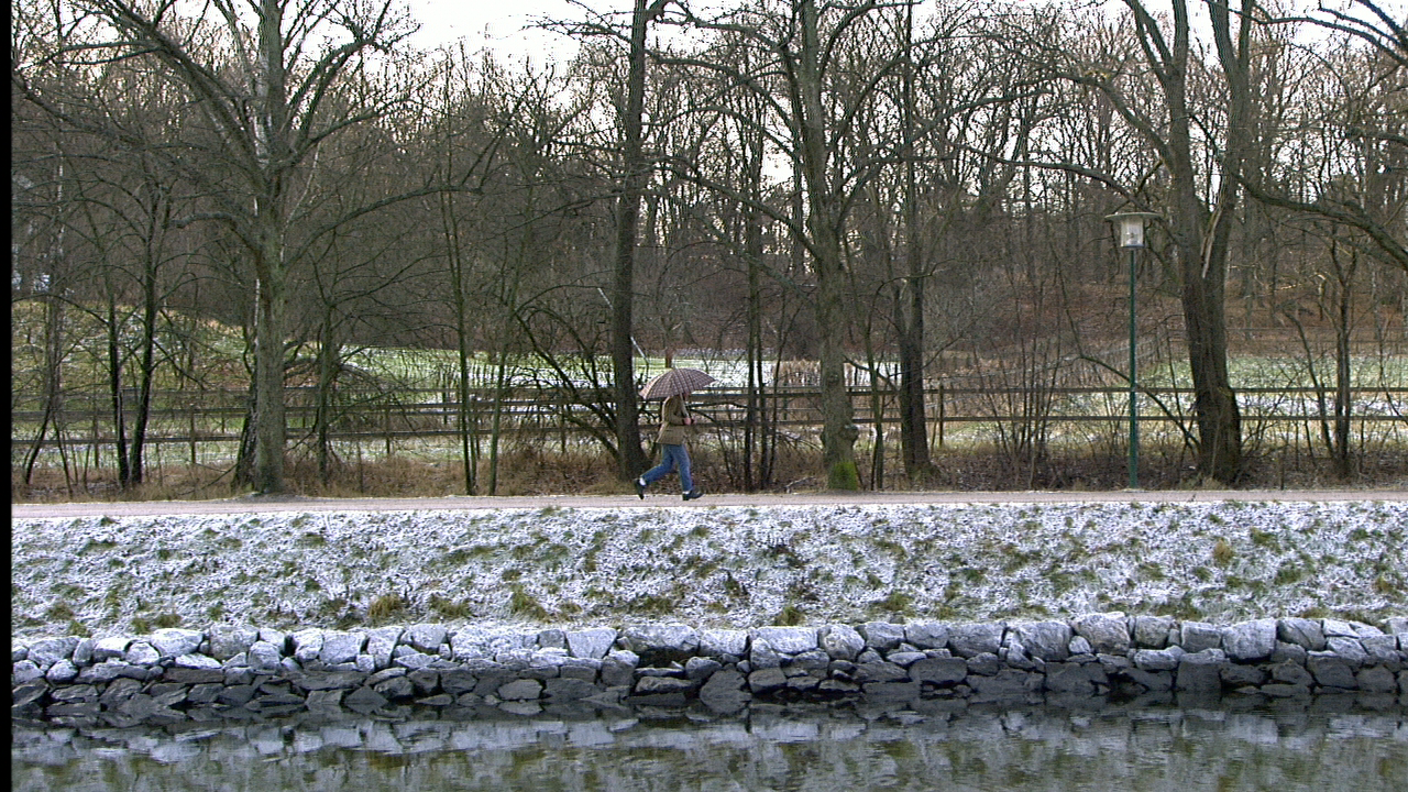
This is the effect that activity masking makes on an image. The effect is most visible in the low-contrast areas, such as the small branches in the background.
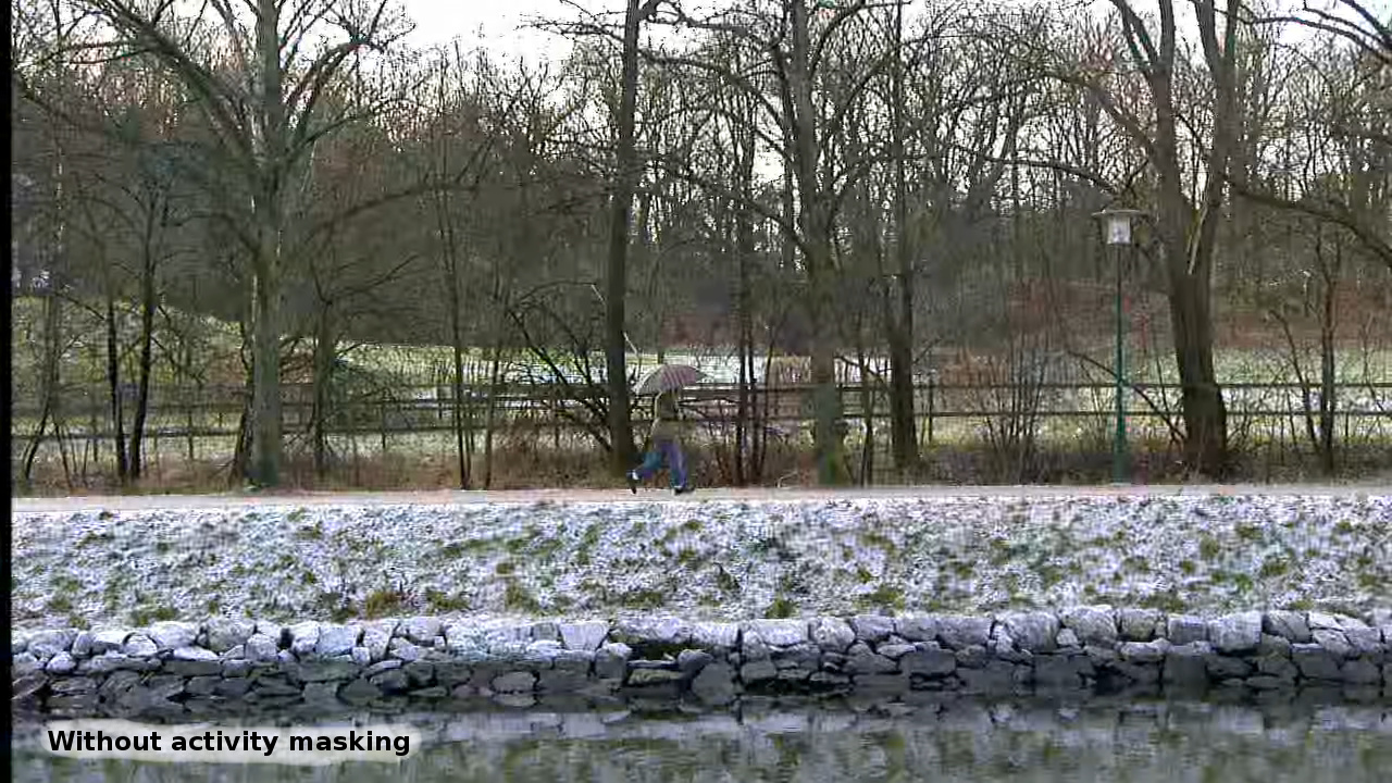
Interestingly, according to the commonly used PSNR metric, the "no activity masking" image is better by about 0.5 dB, despite losing lots of the details. That's because PVQ with activity masking takes bits away from less important areas to move them to more important areas — just like audio codecs have been doing since the 80s. It's just that audio coding people have given up entirely on SNR-derived metrics, whereas for many reasons (some of which are partially valid), video coding folks still use them.
Putting everything together, here's how Daala with PVQ and activity masking compares to JPEG at equal rate.


Perceptual Vector Quantization has been enabled by default in Daala for some time now. All the code can be found in the Daala git repository, in the pvq*.c files. It is the only quantization method since the removal of all scalar quantization code. There is still a lot of work left to do though. First, PVQ comes with dozens of tuning knobs that impact the final quality. Second, most of the code related to Householder and gain companding is still using floating-point computation, which we definitely do not want to have in the final codec, but is currently making development easier.
This demo is intentionally as light as possible on the math details. More details are available in this Perceptual Vector Quantization for Video Coding, presented at the SPIE Visual Information Processing and Communication Conference.
—Jean-Marc Valin (jmvalin@jmvalin.ca) November 18, 2014